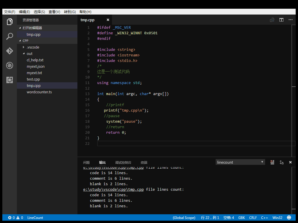
The LineCount extension for Visual Studio Code counts and displays the lines of code, the lines of comment, the lines of blank.
Features
Count current file.
Count workspace files, you can custom the includes/excludes file pattern.
Support languages: c,cpp,java,js,ts,cs(//,/*,*/),sql(--,/*,*/),pas(//,{*,*}),perl(#,=pod,=cut),ruby(#,=begin,=end),python(#,'''),vb('),html(<!--,-->),bat(::),sh(#),ini(;),fortran(!),m(%).
You can customize the comment symbol, add new languages support.
Line number information can be output to JSON, TXT, CSV, Markdown file.
Installs
ext install linecount
Through Code
Download source code and install dependencies:
git clone https://github.com/yycalm/linecount.git
cd linecount
npm install
code .
Extension Settings
LineCount.showStatusBarItem: (boolean|default true) Show/hide the status bar item for LineCount commands.
LineCount.comment.separator.blockend: (string |default none) Block end comment symbol.
LineCount.comment.separator.blocktol: (boolean |default false) Whether the block comment must be started on the line.
LineCount.comment.separator.string.doublequotes: (boolean |default true) String using double quotes.
LineCount.comment.separator.string.singlequotes: (boolean |default true) String using single quotes.
LineCount configuration examples:
send_email(destinaiton, subject=" ", msg=" "):
    '''
    Arguements:
        destination: Takes in destionation email of type string
        subject(optional arguement): Takes in a string as an input (Default arg: None)
        msg(optional arguement): Takes in a message of type string as input (Default arg: None)
    '''
Sends an email with attachment(s) included.
send_email_with_attachment(destination, files, sub="Subject", text="No text"):
''' Arguements: destination: Takes in destionation email of type string files: Take in a list of strings as input sub(optional arguement): Takes in a string as an input (default arg empty) text(optional arguement): Takes in a message of type string as input (default arg empty) '''
Usage
Make sure you have Python 3.6 or 3.7 installed. Then, import the library from TestPyPi (Test Python Packaging Index)
pipinstall-ihttps://test.pypi.org/simple/pynotify
A demo script of this in action is shown below
frompynotifyimportsend_email, send_email_with_attachmentsubject="Killer Robot"message="Hi there!"dest="youremail@youremail.com"# add your email here# attachment paths are stored in an arrayimage= ["cat.jpg"] # for one fileimages= ["cat.jpg", "dog.jpg"] # for multiple files# sends an emailsend_email(dest, "Hello!")
# sends an email with attachementssend_email_with_attachment(dest, images, subject, message)
Takeaways
Program written in Python 3.6
Nothing here. What did you expect? A cookie!?
Need to update dummy google account to less secure if not used for a long time, as google automatically shuts it down!
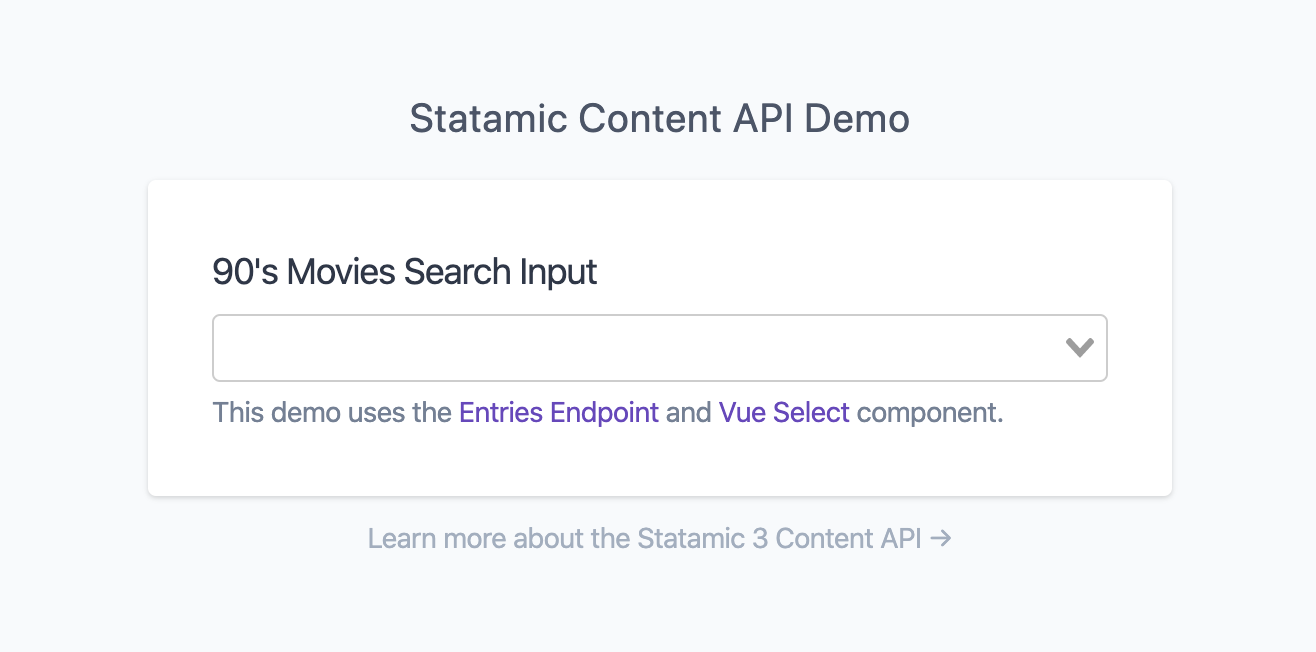
Statamic 3 is the very latest and greatest version of Statamic, a uniquely powerful CMS built on Laravel and designed to make building and managing bespoke websites radically efficient and remarkably enjoyable.
Demo Details
This Content API Demo uses the entries endpoint on a Movies collection to fetch and and filter data with the help of Vue Select.
The returned data from the /api/collections/movies/entries call is rendered in the home.antlers.html template, inside a scoped slot for the Vue Select component.
Screenshot
Want to try it for yourself?
1. Clone the project repo locally and install the dependencies.
git clone git@github.com:statamic/content-api-demo.git
cd content-api-demo
composer install
npm i && npm run dev
cp .env.example .env && php artisan key:generate
2. Visit content-api-demo.test (or whatever your dev URL pattern is) to see it in action
3. Make a new user – If you want to mess around and create/modify entries. You’ll want it to be a super so you have access to everything.
NaDyNet is a MATLAB-based GUI software designed for analysing task-based fMRI data under naturalistic stimuli (also applicable to resting-state fMRI data), aiming to advance naturalistic scene neuroscience.
Naturalistic stimuli refer to rich and continuous stimuli such as watching movies or listening to stories. This paradigm represents an emerging trend in brain science research. Unlike block or event-related designs, continuous-stimulus fMcRI signals are challenging to analyse using traditional GLM methods. NaDyNet provides dynamic analysis methods capable of real-time brain network and activation analysis.
Naturalistic stimuli refer to rich and continuous stimuli such as watching movies or listening to stories. This paradigm represents an emerging trend in brain science research. Unlike block or event-related designs, continuous-stimulus fMRI signals are challenging to analyze using traditional GLM methods. NaDyNet provides dynamic analysis methods capable of real-time brain network and activation analysis.
NaDyNet offers K-means clustering analysis to determine the optimal K value, visualizing multiple clustered states and their corresponding state transition matrices.
2. Hardware and Software Requirements
2.1 Hardware Requirements
This toolbox is a MATLAB-based software for analyzing fMRI (functional magnetic resonance imaging) data. Due to the large size of fMRI data, a minimum of 16GB RAM is required. Methods such as SWISC, CAP, and ISCAP are particularly memory-intensive; for example, the paranoia dataset (22 subjects, 1310 frames per subject) requires 128GB RAM to run. Other methods have lower memory demands.
Additional hardware requirements: Your computer must support MATLAB 2018a or later versions.
2.2 Software Requirements
To run this MATLAB toolbox, the following software environment is required:
Operating System: Windows 7 or later
Network Environment: No specific requirements
Platform: MATLAB 2018a or later
MATLAB Toolboxes: The following toolboxes must be installed:
(1) Medical Imaging Toolbox: A default MATLAB toolbox for image processing (usually pre-installed). Verify its presence by running:
Toolboxes 2–7 can be downloaded via their respective hyperlinks. Alternatively, a bundled download is available here.
After installing the toolbox and its dependencies, add all toolbox paths via MATLAB Home > Set Path. Launch the software by running:
NaDyNet
For convenience, an alias is also supported.
NDN
3. Software Features and Interface
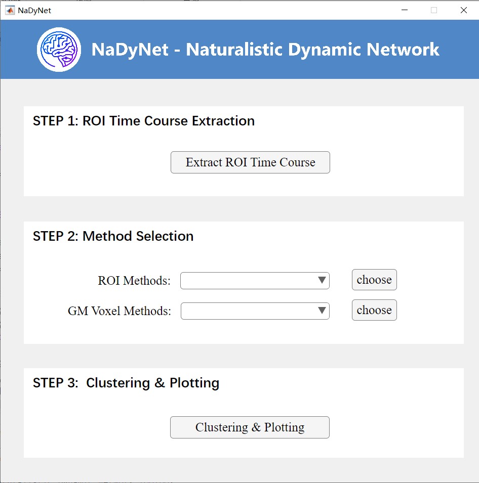
The main interface comprises three modules: Data Extraction, Method Selection, and Clustering & Visualization (Figure 1).
In the ROI TC Extraction Module, we can organize a group of subjects’ fMRI files into a designated folder following a specific naming convention. Then, by selecting a user-defined Regions of Interest (ROI) mask, we extract the ROI time series for these subjects and save them to a user-specified output path.
In the Method Selection Module, two analysis approaches are available:
ROI-Based Methods: These methods focus on predefined regions of interest (ROIs) for dynamic brain network analysis.
Grey Matter Voxel-Based Methods: These methods analyze the entire brain or grey matter at the voxel level.
If you choose the Grey Matter Voxel-Based Method, you can skip the first step (ROI time series extraction).
Clustering & Plotting Module:
Use the Best K function to determine the optimal number of clusters (K).
Alternatively, manually set a K value to perform clustering on dynamic brain network analysis results.
The tool will generate K cluster centers (states), visualize them, and plot the state transition matrix for the subject group.
Figure 1. Main Interface
**3.1 **Data Extraction Module
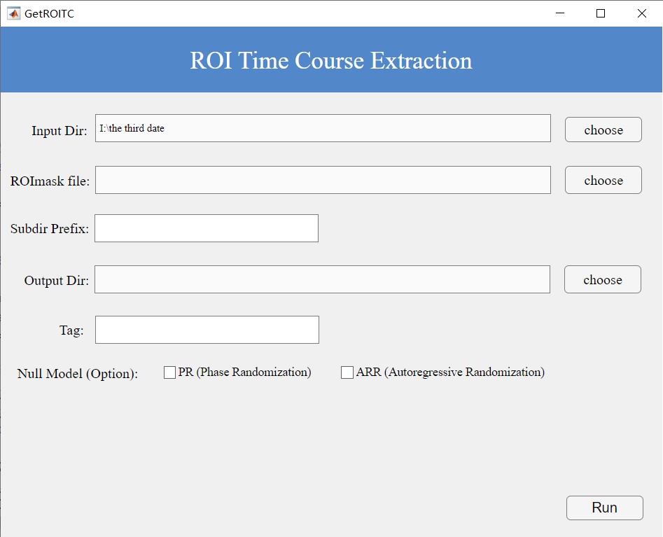
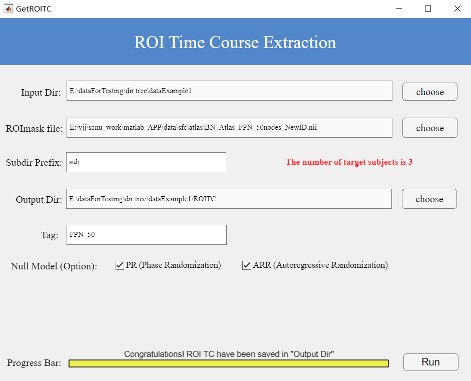
Click Extract ROI Time Course in Step 1 to access this module (Figure 2).
Figure 2. ROI Time Course Extraction Interface
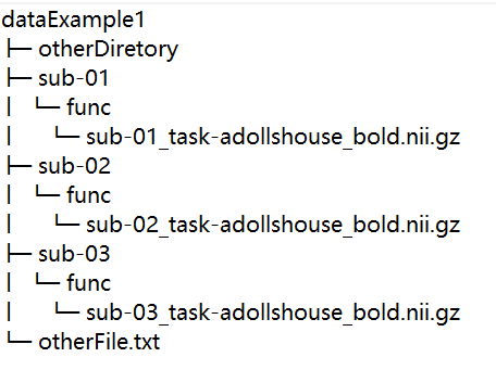
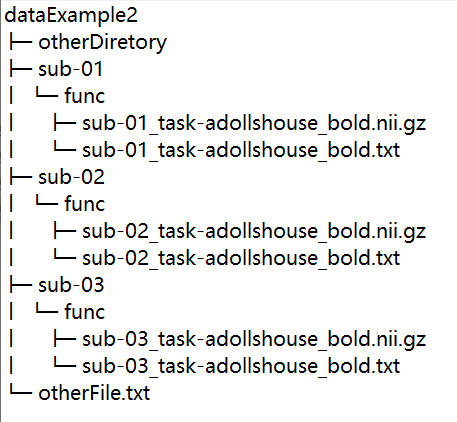
Subject data should follow the BIDS standard (Figure 3):
Each subject (e.g., sub01, sub02) has a dedicated folder containing fMRI files (preprocessed) , with .nii.gz and .nii extensions supported, in a func subdirectory.
Folder names must share a common prefix (e.g., sub).
Figure 3. Input File Structure
Steps:
ROI Mask: Select a mask file (must match fMRI voxel dimensions).
Subject Prefix: Enter the common prefix (e.g., sub); the interface will display the detected subject count (Figure 4).
After correctly entering all required parameters as described above, click the “Run” button to execute the process. Upon successful completion, as shown at the bottom of Figure 4, you will be notified that the results have been saved to your specified output folder.
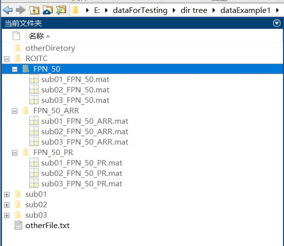
For each subject, a corresponding .mat file containing the ROI time series will be generated. This file contains a two-dimensional matrix where:
Rows represent the number of time points
Columns represent the number of ROIs
If you have selected the null model option, additional subfolders (PR or ARR) will be automatically created to store the generated null model data. The output structure is illustrated in Figure 5.
Note: The software will preserve all original data while creating these additional null model datasets when the corresponding option is enabled.
Figure 5. ROI TC Output Files
3.2 Method Selection Module
The method selection module includes two analytical approaches: ROI-based methods and grey matter voxel-based methods.
3.2.1 ROI-Based Methods
The software implements 12 ROI-based analysis methods, of which 10 are dynamic and the remaining 2 are static:
Core Dynamic Methods:
Dynamic Conditional Correlation (DCC)
Sliding-Window Functional Connectivity with L1-regularization (SWFC)
Flexible Least Squares (FLS)
Generalized Linear Kalman Filter (GLKF)
Multiplication of Temporal Derivatives (MTD)
Enhanced Inter-Subject Versions:
Inter-Subject DCC (ISDCC)
Inter-Subject SWFC (ISSWFC)
Inter-Subject FLS (ISFLS)
Inter-Subject GLKF (ISGLKF)
Inter-Subject MTD (ISMTD)
Static Method:
Static Functional Connectivity (SFC)
Inter-subject Functional Connectivity (ISFC)
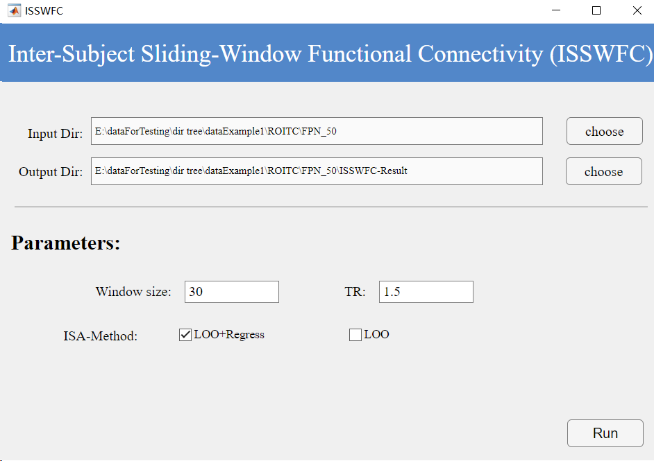
Figure 6. ISSWFC Interface
Workflow:
1. Input Path Selection
Path Requirement: Select the folder containing outputs from Step 1. Note: The selected directory must not contain any other .mat files unrelated to the analysis.
2. Output Path Specification
Options:
Manually specify a custom save path.
Use the default path (as shown in Figure 6).
3. Parameter Input Rules
For SFC and ISFC : No additional parameters required. Proceed directly to execution.
For Other 10 Methods: Mandatory parameter input (see Figure 6). Below are detailed descriptions:
Method-Specific Parameters
1. DCC (Dynamic Conditional Correlation)
TR (Repetition Time):
Definition: Time interval between consecutive fMRI volume acquisitions.
Value Range: Must be >0.
Unit: Seconds.
2. SWFC (Sliding-Window Functional Connectivity)
winSize (Window Size):
Definition: Duration of the sliding window for dynamic FC calculation.
Unit: TR
Typical Range: [20, 40] TRs.
Constraints: Must be >1 and < total TR count.
TR: As above.
3. FLS (Flexible Least Squares)
mu (Penalty Weight):
Definition: Regularization coefficient balancing model fit and smoothness.
Default: 100.
TR: As above.
4. GLKF (Generalized Linear Kalman Filter)
pKF (Model Order):
Definition: Lag order of the multivariate autoregressive (MVAR) model.
Format: Plain text files with .txt or .csv extension
Temporal requirement: Must precisely match fMRI scan duration
Default behavior: System assumes zero motion when files are absent
Note: Only required for CAP/ISCAP analyses (optional for ISC/SWISC)
Figure 8. Input Structure for Voxel-Based Methods
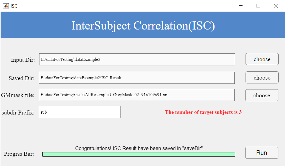
ISC Workflow (Figure 9):
Input Directory: Path to organized subject data.
Grey Matter Mask: Must match fMRI voxel dimensions.
Subject Prefix: Enter common prefix (e.g., sub). Since all subject folders follow a standardized naming convention with the common prefix ‘sub’, simply entering this prefix will automatically display the number of identified subjects in the interface.
Figure 9. ISC Interface
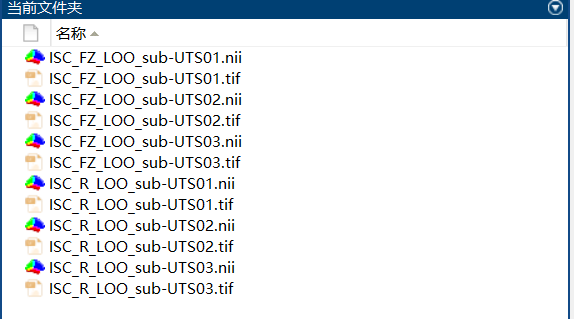
Two 3D NII files per subject (raw ISC and Fisher’s Z-transformed). With BrainNet Viewer installed, .tif images are also generated (Figure 10).
Figure 10. ISC Output
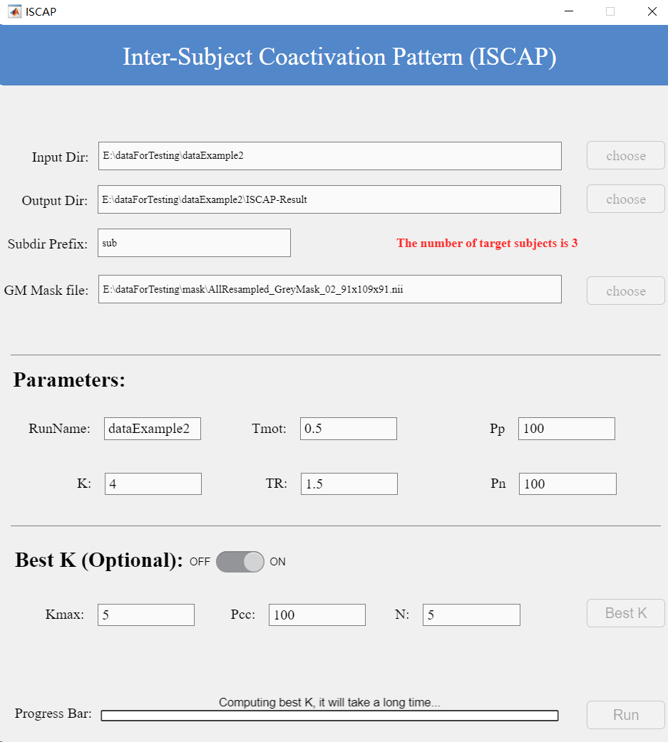
ISCAP Workflow (Figure 11)
(1) After organizing the data according to the rules shown in Figure 8, set the data directory as the input path.
(2) Select a gray matter mask with voxel dimensions matching the source data.
(3) Since subject folders follow a consistent naming pattern with the common prefix ‘sub’, simply enter this prefix and the interface will display the number of detected subjects.
(4) Then input appropriate ISCAP parameters on the page:
RunName: Identifies the current subject group dataset.
Tmot: Motion threshold; frames exceeding this value in motion files will be excluded.
K: Number of clusters (typically 1-12).
TR: Repetition Time.
pN/pP: Percentage of positive/negative voxels retained for clustering (range: [1,100]); remaining voxels are set to zero.
Determine the optimal K value using consensus clustering.
Note: This step is computationally intensive and memory-demanding. Run it only if necessary.
Kmax: Range [3, 12]. The toolbox will search for the best K within [2, Kmax].
Pcc: Range [80, 100], the percentage of original data retained. Recommended: 100 (smaller values may cause errors but can reduce computation if successful).
N: Number of iterations.
After obtaining the optimal K, input it as K and click Run to execute ISCAP.
Figure 11. ISCAP Interface
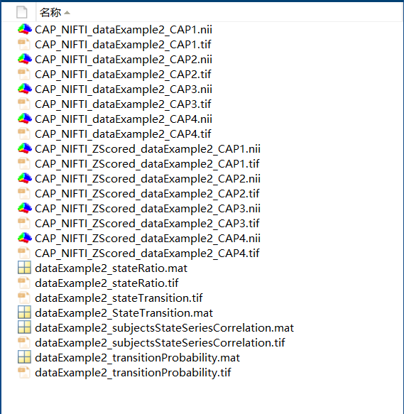
After entering these parameters correctly, click Run. Upon successful execution (as shown at the bottom of Figure 11), results will be saved in the specified output folder. Each subject’s ISCAP results include:
Two 3D NII files: raw ISCAP results and Z-scored versions.
A state transition matrix (.mat file) with corresponding visualization.
Proportion of each state across all subjects after clustering
Transition probabilities between states
Correlation of state sequences for each subject
As shown in Figure 12, if BrainNet Viewer is installed in MATLAB, each 3D file will generate a corresponding TIF image.
Figure 12. ISCAP Output
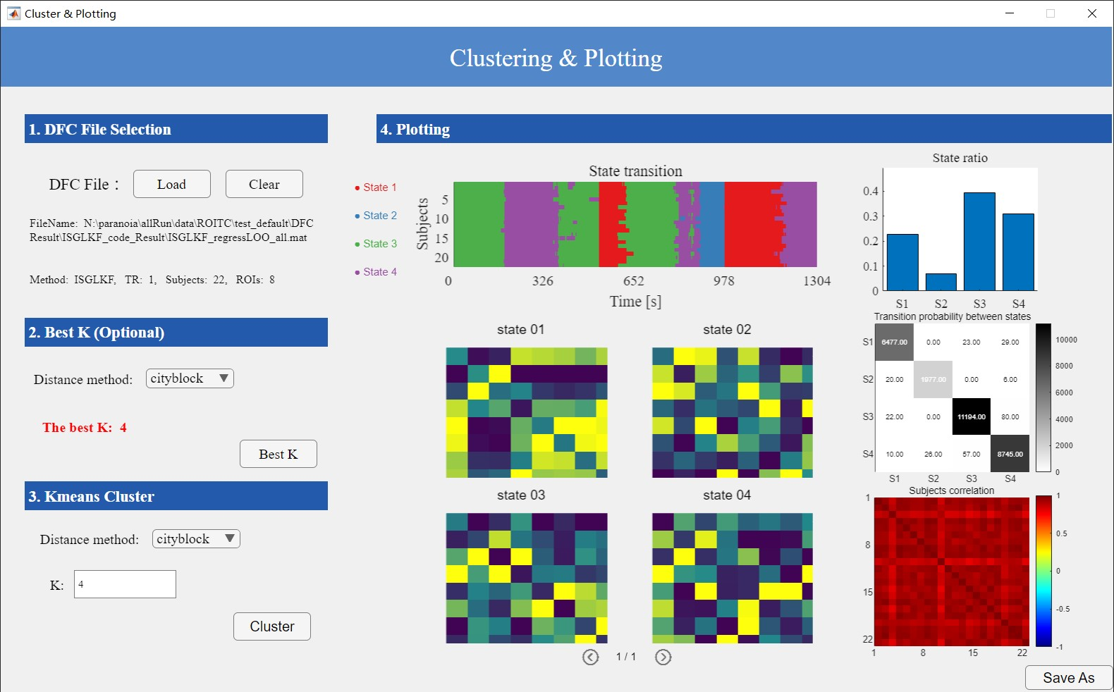
3.3. Clustering and Plotting Module
This interface consists of four components: data input, optimal K value calculation, K-means clustering analysis, and visualization (Figure 13).
Figure 13. Clustering and Plotting Interface
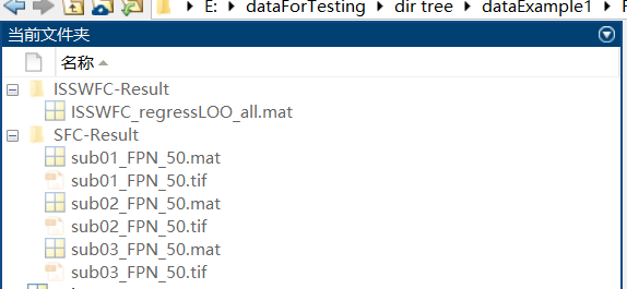
Data Input: Users need to input files ending with _all.mat, which contain results from dynamic ROI analysis methods (file location shown in Figure 7). The interface will display file details automatically.
Optimal K Calculation: Select a distance metric for clustering and click “Best K” to compute and display the optimal K value.
K-means Clustering:
Use either the computed optimal K or manually specify a K value
Select a clustering distance metric
Click “Cluster” to perform K-means clustering and generate the following visualizations (Figure 14):
K state matrices (size: nROI × nROI)
State transition matrix (size: nSub × nT; x-axis in seconds, max = nT × TR)
Proportion of each state across all subjects
Transition probabilities between states
Correlation of state sequences for each subject (matrix size: nSub × nSub)
Figure 14. Clustering and Plotting Results
Output:
Saved visualization images
Dynamic functional connectivity (DFC) variability for each subject (saved in “variability” folder)
An output file (Figure 15)
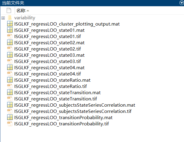
Figure 15. Output Data from Clustering and Plotting
The _output.mat file contains:
info: Input data information
plotting: Source data for visualizations (K clustered state matrices, subject correlation matrices, state proportions, transition probabilities)
clusterInfo: Clustering parameters (distance metric, K value)
stateTransition: State transition matrices for all subjects
NaDyNet is a MATLAB-based GUI software designed for analysing task-based fMRI data under naturalistic stimuli (also applicable to resting-state fMRI data), aiming to advance naturalistic scene neuroscience.
Naturalistic stimuli refer to rich and continuous stimuli such as watching movies or listening to stories. This paradigm represents an emerging trend in brain science research. Unlike block or event-related designs, continuous-stimulus fMcRI signals are challenging to analyse using traditional GLM methods. NaDyNet provides dynamic analysis methods capable of real-time brain network and activation analysis.
Naturalistic stimuli refer to rich and continuous stimuli such as watching movies or listening to stories. This paradigm represents an emerging trend in brain science research. Unlike block or event-related designs, continuous-stimulus fMRI signals are challenging to analyze using traditional GLM methods. NaDyNet provides dynamic analysis methods capable of real-time brain network and activation analysis.
NaDyNet offers K-means clustering analysis to determine the optimal K value, visualizing multiple clustered states and their corresponding state transition matrices.
2. Hardware and Software Requirements
2.1 Hardware Requirements
This toolbox is a MATLAB-based software for analyzing fMRI (functional magnetic resonance imaging) data. Due to the large size of fMRI data, a minimum of 16GB RAM is required. Methods such as SWISC, CAP, and ISCAP are particularly memory-intensive; for example, the paranoia dataset (22 subjects, 1310 frames per subject) requires 128GB RAM to run. Other methods have lower memory demands.
Additional hardware requirements: Your computer must support MATLAB 2018a or later versions.
2.2 Software Requirements
To run this MATLAB toolbox, the following software environment is required:
Operating System: Windows 7 or later
Network Environment: No specific requirements
Platform: MATLAB 2018a or later
MATLAB Toolboxes: The following toolboxes must be installed:
(1) Medical Imaging Toolbox: A default MATLAB toolbox for image processing (usually pre-installed). Verify its presence by running:
Toolboxes 2–7 can be downloaded via their respective hyperlinks. Alternatively, a bundled download is available here.
After installing the toolbox and its dependencies, add all toolbox paths via MATLAB Home > Set Path. Launch the software by running:
NaDyNet
For convenience, an alias is also supported.
NDN
3. Software Features and Interface
The main interface comprises three modules: Data Extraction, Method Selection, and Clustering & Visualization (Figure 1).
In the ROI TC Extraction Module, we can organize a group of subjects’ fMRI files into a designated folder following a specific naming convention. Then, by selecting a user-defined Regions of Interest (ROI) mask, we extract the ROI time series for these subjects and save them to a user-specified output path.
In the Method Selection Module, two analysis approaches are available:
ROI-Based Methods: These methods focus on predefined regions of interest (ROIs) for dynamic brain network analysis.
Grey Matter Voxel-Based Methods: These methods analyze the entire brain or grey matter at the voxel level.
If you choose the Grey Matter Voxel-Based Method, you can skip the first step (ROI time series extraction).
Clustering & Plotting Module:
Use the Best K function to determine the optimal number of clusters (K).
Alternatively, manually set a K value to perform clustering on dynamic brain network analysis results.
The tool will generate K cluster centers (states), visualize them, and plot the state transition matrix for the subject group.
Figure 1. Main Interface
**3.1 **Data Extraction Module
Click Extract ROI Time Course in Step 1 to access this module (Figure 2).
Figure 2. ROI Time Course Extraction Interface
Subject data should follow the BIDS standard (Figure 3):
Each subject (e.g., sub01, sub02) has a dedicated folder containing fMRI files (preprocessed) , with .nii.gz and .nii extensions supported, in a func subdirectory.
Folder names must share a common prefix (e.g., sub).
Figure 3. Input File Structure
Steps:
ROI Mask: Select a mask file (must match fMRI voxel dimensions).
Subject Prefix: Enter the common prefix (e.g., sub); the interface will display the detected subject count (Figure 4).
After correctly entering all required parameters as described above, click the “Run” button to execute the process. Upon successful completion, as shown at the bottom of Figure 4, you will be notified that the results have been saved to your specified output folder.
For each subject, a corresponding .mat file containing the ROI time series will be generated. This file contains a two-dimensional matrix where:
Rows represent the number of time points
Columns represent the number of ROIs
If you have selected the null model option, additional subfolders (PR or ARR) will be automatically created to store the generated null model data. The output structure is illustrated in Figure 5.
Note: The software will preserve all original data while creating these additional null model datasets when the corresponding option is enabled.
Figure 5. ROI TC Output Files
3.2 Method Selection Module
The method selection module includes two analytical approaches: ROI-based methods and grey matter voxel-based methods.
3.2.1 ROI-Based Methods
The software implements 12 ROI-based analysis methods, of which 10 are dynamic and the remaining 2 are static:
Core Dynamic Methods:
Dynamic Conditional Correlation (DCC)
Sliding-Window Functional Connectivity with L1-regularization (SWFC)
Flexible Least Squares (FLS)
Generalized Linear Kalman Filter (GLKF)
Multiplication of Temporal Derivatives (MTD)
Enhanced Inter-Subject Versions:
Inter-Subject DCC (ISDCC)
Inter-Subject SWFC (ISSWFC)
Inter-Subject FLS (ISFLS)
Inter-Subject GLKF (ISGLKF)
Inter-Subject MTD (ISMTD)
Static Method:
Static Functional Connectivity (SFC)
Inter-subject Functional Connectivity (ISFC)
Figure 6. ISSWFC Interface
Workflow:
1. Input Path Selection
Path Requirement: Select the folder containing outputs from Step 1. Note: The selected directory must not contain any other .mat files unrelated to the analysis.
2. Output Path Specification
Options:
Manually specify a custom save path.
Use the default path (as shown in Figure 6).
3. Parameter Input Rules
For SFC and ISFC : No additional parameters required. Proceed directly to execution.
For Other 10 Methods: Mandatory parameter input (see Figure 6). Below are detailed descriptions:
Method-Specific Parameters
1. DCC (Dynamic Conditional Correlation)
TR (Repetition Time):
Definition: Time interval between consecutive fMRI volume acquisitions.
Value Range: Must be >0.
Unit: Seconds.
2. SWFC (Sliding-Window Functional Connectivity)
winSize (Window Size):
Definition: Duration of the sliding window for dynamic FC calculation.
Unit: TR
Typical Range: [20, 40] TRs.
Constraints: Must be >1 and < total TR count.
TR: As above.
3. FLS (Flexible Least Squares)
mu (Penalty Weight):
Definition: Regularization coefficient balancing model fit and smoothness.
Default: 100.
TR: As above.
4. GLKF (Generalized Linear Kalman Filter)
pKF (Model Order):
Definition: Lag order of the multivariate autoregressive (MVAR) model.
Format: Plain text files with .txt or .csv extension
Temporal requirement: Must precisely match fMRI scan duration
Default behavior: System assumes zero motion when files are absent
Note: Only required for CAP/ISCAP analyses (optional for ISC/SWISC)
Figure 8. Input Structure for Voxel-Based Methods
ISC Workflow (Figure 9):
Input Directory: Path to organized subject data.
Grey Matter Mask: Must match fMRI voxel dimensions.
Subject Prefix: Enter common prefix (e.g., sub). Since all subject folders follow a standardized naming convention with the common prefix ‘sub’, simply entering this prefix will automatically display the number of identified subjects in the interface.
Figure 9. ISC Interface
Two 3D NII files per subject (raw ISC and Fisher’s Z-transformed). With BrainNet Viewer installed, .tif images are also generated (Figure 10).
Figure 10. ISC Output
ISCAP Workflow (Figure 11)
(1) After organizing the data according to the rules shown in Figure 8, set the data directory as the input path.
(2) Select a gray matter mask with voxel dimensions matching the source data.
(3) Since subject folders follow a consistent naming pattern with the common prefix ‘sub’, simply enter this prefix and the interface will display the number of detected subjects.
(4) Then input appropriate ISCAP parameters on the page:
RunName: Identifies the current subject group dataset.
Tmot: Motion threshold; frames exceeding this value in motion files will be excluded.
K: Number of clusters (typically 1-12).
TR: Repetition Time.
pN/pP: Percentage of positive/negative voxels retained for clustering (range: [1,100]); remaining voxels are set to zero.
Determine the optimal K value using consensus clustering.
Note: This step is computationally intensive and memory-demanding. Run it only if necessary.
Kmax: Range [3, 12]. The toolbox will search for the best K within [2, Kmax].
Pcc: Range [80, 100], the percentage of original data retained. Recommended: 100 (smaller values may cause errors but can reduce computation if successful).
N: Number of iterations.
After obtaining the optimal K, input it as K and click Run to execute ISCAP.
Figure 11. ISCAP Interface
After entering these parameters correctly, click Run. Upon successful execution (as shown at the bottom of Figure 11), results will be saved in the specified output folder. Each subject’s ISCAP results include:
Two 3D NII files: raw ISCAP results and Z-scored versions.
A state transition matrix (.mat file) with corresponding visualization.
Proportion of each state across all subjects after clustering
Transition probabilities between states
Correlation of state sequences for each subject
As shown in Figure 12, if BrainNet Viewer is installed in MATLAB, each 3D file will generate a corresponding TIF image.
Figure 12. ISCAP Output
3.3. Clustering and Plotting Module
This interface consists of four components: data input, optimal K value calculation, K-means clustering analysis, and visualization (Figure 13).
Figure 13. Clustering and Plotting Interface
Data Input: Users need to input files ending with _all.mat, which contain results from dynamic ROI analysis methods (file location shown in Figure 7). The interface will display file details automatically.
Optimal K Calculation: Select a distance metric for clustering and click “Best K” to compute and display the optimal K value.
K-means Clustering:
Use either the computed optimal K or manually specify a K value
Select a clustering distance metric
Click “Cluster” to perform K-means clustering and generate the following visualizations (Figure 14):
K state matrices (size: nROI × nROI)
State transition matrix (size: nSub × nT; x-axis in seconds, max = nT × TR)
Proportion of each state across all subjects
Transition probabilities between states
Correlation of state sequences for each subject (matrix size: nSub × nSub)
Figure 14. Clustering and Plotting Results
Output:
Saved visualization images
Dynamic functional connectivity (DFC) variability for each subject (saved in “variability” folder)
An output file (Figure 15)
Figure 15. Output Data from Clustering and Plotting
The _output.mat file contains:
info: Input data information
plotting: Source data for visualizations (K clustered state matrices, subject correlation matrices, state proportions, transition probabilities)
clusterInfo: Clustering parameters (distance metric, K value)
stateTransition: State transition matrices for all subjects
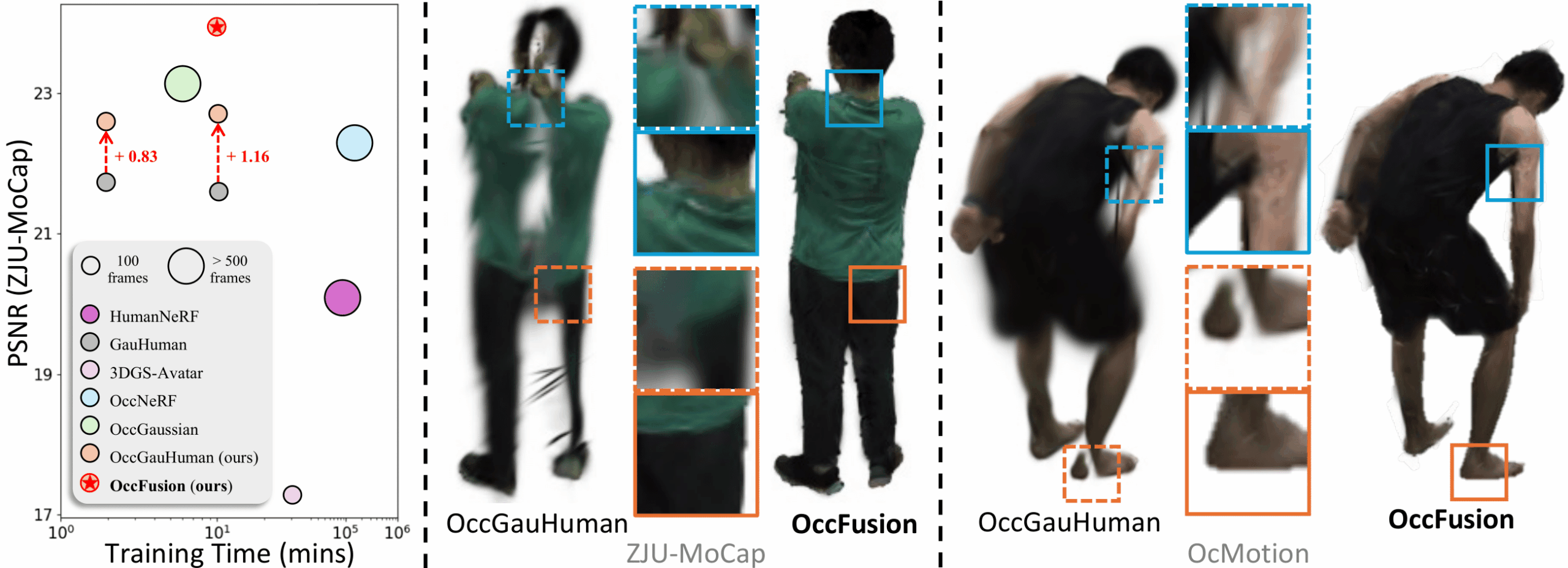
We provide training/rendering code for the 6 OcMotion sequences that are sampled by Wild2Avatar. If you find the preprocessed sequences useful, please consider to cite Wild2Avatar and CHOMP.
Please download the processed sequences here and unzip the downloaded sequences in the ./data/ directory. The structure of ./data/ should look like:
Please register and download the neutral SMPL modelhere. Put the downloaded models in the folder ./assets/.
3. Canonical OpenPose canvas
To enable more efficient canonical space SDS, OpenPose canvas for canonical 2D poses are precomputed and can be downloaded here. Put the downloaded folder in the folder: ./assets/.
(optional) 4. SAM-HQ weights
For training the model in Stage 0 (optional, see below), we need to compute binary masks for complete human inpaintings. We utilized SAM-HQ for segmentation. If you wish to compute the masks on your own, please download the pretrained weights sam_hq_vit_h.pthhere and put the donwloaded weights in the folder: ./assets/.
After successful downloading, the structure of ./assets/ should look like
We provide our pretrained models for all the OcMotion sequences to allow for quick inference/evaluation. Please download the ocmotion/ folder here and put the downloaded folders in ./output/.
Usage
The training of OccFusion consists of 4 sequential stages. Stage 0 and 2 are optional and inpaint the occluded human with customized models, sovlers, and prompts. Different combinations may impact the inpainting results greatly. A high-quality pose conditioned human genertaion is out of the scope of this work. We provide our code (see Stage 0 and Stage 2 below) to allow users to try themselves.
We provide our precomputed generations (to replicate our results in the paper) to be downloaded here. Please unzip and put the oc_generations/ folder directly on the root directory. If you use our computations, Stage 0 and 2 can be skipped.
(optional) Setting Cache Directory for Hugging Face Models
Before training, we highly recommend specifying a customised directory for caching Hugging Face models, which will be downloaded automatically at the first run of the training scripts.
Run Stage 0 (the Initialization Stage) to segment and inpaint binary masks for complete humans with SAM and Stable Diffusion. To run Stage 0 on a OcMotion sequence, uncomment the corresponding SUBJECT variable and
source run_oc_stage0.sh
The segmented binary masks will be saved in the ./oc_genertaions/$SUBJECT/gen_masks/ directory.
Stage 1
Run Stage 1 to start the Optimization Stage. To run Stage 1 on a OcMotion sequence, uncomment the corresponding SUBJECT variable and
source run_oc_stage1.sh
The checkpoint along with renderings will be saved in ./output/$SUBJECT/.
(optional) Stage 2
With an optimized model, run Stage 2 to launch incontext-inpainting. To run Stage 2 on a OcMotion sequence, uncomment the corresponding SUBJECT variable and
source run_oc_stage2.sh
The inpainted RGB images will be saved in the ./oc_genertaions/$SUBJECT/incontext_inpainted/ directory.
Stage 3
Lastly, with the inpainted RGB images and the optimized model checkpoint, run Stage 3 to start the Refinement Stage. To run Stage 3 on a OcMotion sequence, uncomment the corresponding SUBJECT variable and
source run_oc_stage1.sh
The checkpoint along with renderings will be save in ./output/$SUBJECT/.
Rendering
At Stage 1 and 3, a rendering process will be trigered automatically after the training finishes. To explicitly render on a trained checkpoint, run
source render.sh
Acknowledgement
This code base is built upon GauHuman. SDS guidances are borrowed from DreamGaussian.
Check also our prior works on occluded human rendering! OccNeRF and Wild2Avatar.
Citation
If you find this repo useful in your work or research, please cite:
@inproceedings{occfusion,
  title={OccFusion: Rendering Occluded Humans with Generative Diffusion Priors},
  author={Sun, Adam and Xiang, Tiange and Delp, Scott and Fei-Fei, Li and Adeli, Ehsan},
  booktitle={The Thirty-eighth Annual Conference on Neural Information Processing Systems},
  url={https://arxiv.org/abs/2407.00316},
  year={2024}
}